Controlling the grid of penalization levels
David Kepplinger
2026-01-27
Source:vignettes/lambda_grids.Rmd
lambda_grids.RmdThe functions to compute (adaptive) PENSE and PENSEM estimates
automatically select a grid of penalization levels. In many cases, this
grid is well focused on the interesting range of penalization levels,
but sometimes it needs to be adjusted. This guide shows how to adjust
the grid of penalization levels for the the function
adapense_cv(), i.e., for computing adaptive PENSE
estimates. The steps, however, apply to all functions for
computing robust regularized estimates in the pense package (using or
not using cross-validation).
For this guide we first need to load the pense package:
For demonstration purposes, let’s simulate data with 50 observations and 40 available predictors. The error distribution is a heavy-tailed t-distribution and only the first 3 predictors are truly relevant for predicting the response y:
set.seed(1234)
x <- matrix(rweibull(50 * 40, 2, 3), ncol = 40)
y <- 1 * x[, 1] - 1.1 * x[, 2] + 1.2 * x[, 3] + rt(nrow(x), df = 2)
To make the demonstration more realistic, let’s add some contamination to the response value of the first 3 observations and to some predictors:
Adjusting the grid of penalization levels
By default, adapense_cv() creates a grid of 50
penalization levels. The grid spans from the “largest” penalization
level (i.e., the penalization level where the solution is the
intercept-only model) to a multiple of 10-3 of this largest
penalization level.
The number of grid points is controlled with argument
nlambda=. The more grid points, the more models are
explored, but computation time increases accordingly. For most
applications “meaningful” change is only observed between models
differing in at least one predictor.
Particularly in the lower end of the grid, the estimated models often
don’t differ in the number of predictors and exhibit only marginal
differences in the coefficient estimates. This may waste computational
resources on exploring an area of little interest. You can adjust the
lower endpoint of the automatic grid by changing the multiplier with
argument lambda_min_ratio=. The ratio must be less than 1,
and the closer to 1 the narrower the grid. If you need to re-focus the
grid on larger values of the penalization level, you can increase the
ratio, for example, to 0.5:
set.seed(1234)
fit_grid_narrow <- adapense_cv(x, y, alpha = 0.75, lambda_min_ratio = 5e-1, cv_k = 5, cv_repl = 10)
If the model at the lowest penalization level is still fairly sparse and the best model seems to be in this range, you may need to decrease the ratio, e.g., to 0.05:
set.seed(1234)
fit_grid_wide <- adapense_cv(x, y, alpha = 0.75, lambda_min_ratio = 5e-2, cv_k = 5, cv_repl = 10)
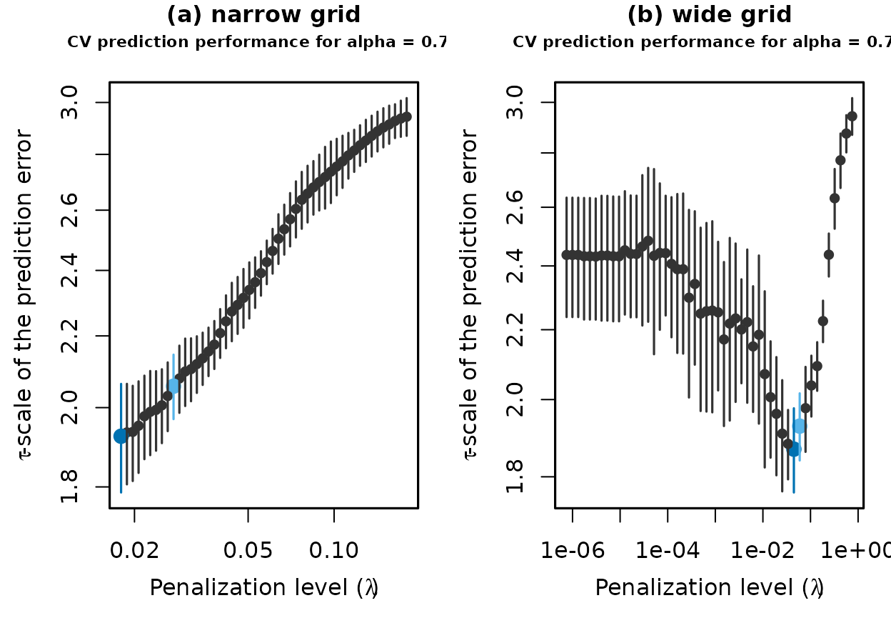
Prediction performance of models estimated on different grids of the
penalization level: (a) narrow grid with
lambda_min_ratio=1e-1, (b) wide grid with
lambda_min_ratio=1e-6.
From these plots we can see that the grid in the left plot is too narrow, as a smaller penalization level than 0.02 would likely lead to a better predictive model. On the right, however, the grid is too wide. Penalization levels less than 0.01 seam to have substantially worse prediction accuracy. Therefore, we can compute adaptive PENSE estimates on a better focused grid with:
set.seed(1234)
fit_grid_focused <- adapense_cv(x, y, alpha = 0.75, lambda_min_ratio = 1e-1, cv_k = 5, cv_repl = 10)
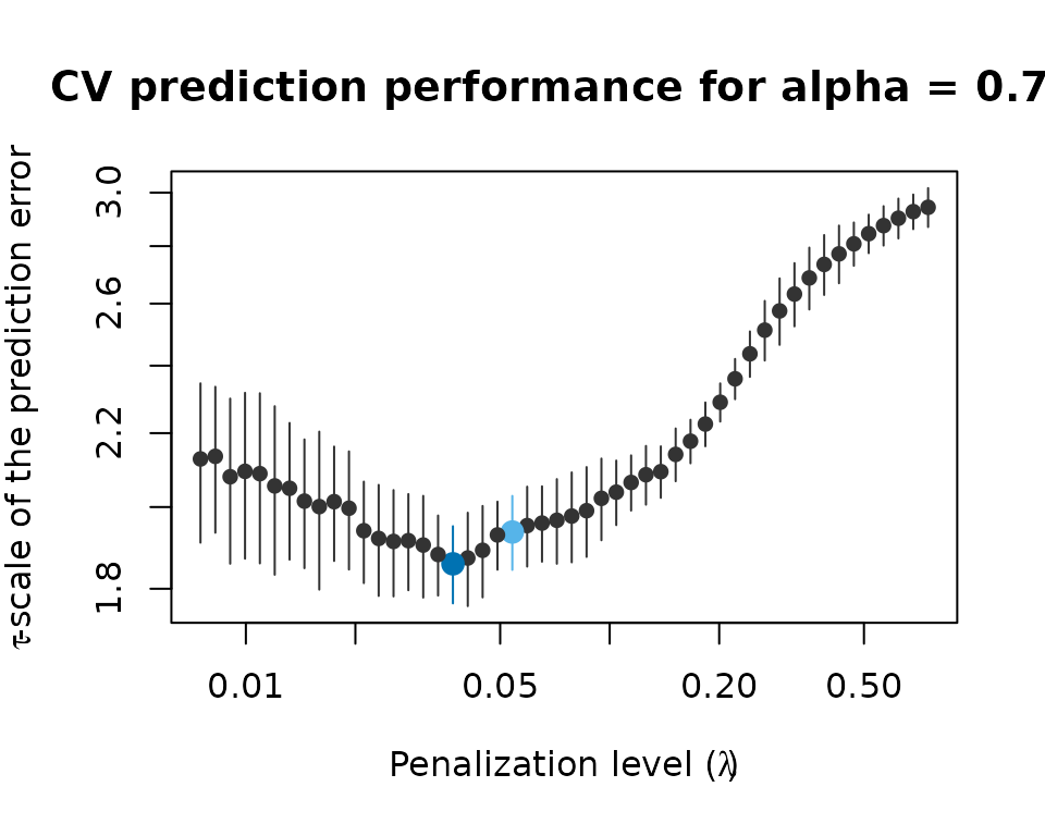
Indeed, the plot shows that the range of interest (around the minimum) is covered by several penalization levels:

Prediction performance of models estimated over a well-focused grid of penalization levels.
Manually supplying a grid of penalization levels
The function adapense_cv() and friends also allows you
to specify your own grid of penalization levels via the
lambda= argument.
Note that for adapense_cv() the argument
lambda= applies to both the preliminary PENSE estimate and
the adaptive PENSE estimate. In most cases, however, this is not what
you want. A sensible grid of penalization levels for the preliminary
estimate is in general quite different from a good grid of penalization
levels for the adaptive estimate.
To compute adaptive PENSE estimates with separately specified manual grids for the preliminary and the adaptive PENSE estimates, you need to compute them manually via
fit_preliminary <- pense_cv(x, y, alpha = 0, cv_k = 5, cv_repl = 10,
                            lambda = exp(seq(log(0.5), log(20), length.out = 5)))
exponent <- 1
penalty_loadings <- 1 / abs(coef(fit_preliminary)[-1])^exponent
fit_adaptive <- pense_cv(x, y, alpha = 0.75, cv_k = 5, cv_repl = 10,
                         lambda = exp(seq(log(0.1), log(2), length.out = 5)))
summary(fit_adaptive)
#> PENSE fit with prediction performance estimated by 10 replications of 5-fold
#> ris cross-validation.
#>
#> 8 out of 40 predictors have non-zero coefficients:
#>
#>                Estimate
#> (Intercept)  1.56453280
#> X1           0.41947742
#> X2          -0.49314705
#> X3           0.41263669
#> X5           0.05041418
#> X26         -0.08230093
#> X29          0.03015557
#> X36         -0.07564768
#> X39         -0.03997095
#> ---
#>
#> Hyper-parameters: lambda=0.9457416, alpha=0.75