Plot the coefficient path for fitted penalized elastic net S- or LS-estimates of regression.
Usage
# S3 method for class 'pense_fit'
plot(x, alpha, ...)See also
Other functions for plotting and printing:
plot.pense_cvfit(),
prediction_performance(),
summary.pense_cvfit()
Examples
# Compute the PENSE regularization path for Freeny's revenue data
# (see ?freeny)
data(freeny)
x <- as.matrix(freeny[ , 2:5])
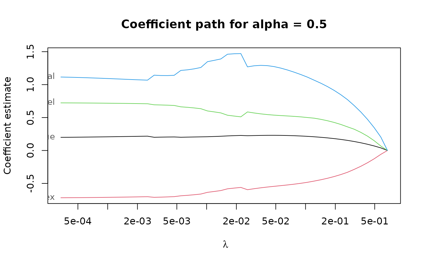
regpath <- pense(x, freeny$y, alpha = 0.5)
plot(regpath)
 # Extract the coefficients at a certain penalization level
coef(regpath, lambda = regpath$lambda[[1]][[40]])
#> (Intercept) lag.quarterly.revenue price.index
#> -6.5082299 0.2510560 -0.6879670
#> income.level market.potential
#> 0.7090986 0.9409940
# What penalization level leads to good prediction performance?
set.seed(123)
cv_results <- pense_cv(x, freeny$y, alpha = 0.5,
cv_repl = 2, cv_k = 4)
plot(cv_results, se_mult = 1)
# Extract the coefficients at a certain penalization level
coef(regpath, lambda = regpath$lambda[[1]][[40]])
#> (Intercept) lag.quarterly.revenue price.index
#> -6.5082299 0.2510560 -0.6879670
#> income.level market.potential
#> 0.7090986 0.9409940
# What penalization level leads to good prediction performance?
set.seed(123)
cv_results <- pense_cv(x, freeny$y, alpha = 0.5,
cv_repl = 2, cv_k = 4)
plot(cv_results, se_mult = 1)
 # Print a summary of the fit and the cross-validation results.
summary(cv_results)
#> PENSE fit with prediction performance estimated by 2 replications of 4-fold ris
#> cross-validation.
#>
#> 4 out of 4 predictors have non-zero coefficients:
#>
#> Estimate
#> (Intercept) -4.7921541
#> X1 0.3338834
#> X2 -0.6140406
#> X3 0.6954769
#> X4 0.7316339
#> ---
#>
#> Hyper-parameters: lambda=0.0003364066, alpha=0.5
# Extract the coefficients at the penalization level with
# smallest prediction error ...
coef(cv_results)
#> (Intercept) lag.quarterly.revenue price.index
#> -4.7921541 0.3338834 -0.6140406
#> income.level market.potential
#> 0.6954769 0.7316339
# ... or at the penalization level with prediction error
# statistically indistinguishable from the minimum.
coef(cv_results, lambda = '1-se')
#> (Intercept) lag.quarterly.revenue price.index
#> -11.4754472 0.2265866 -0.5739724
#> income.level market.potential
#> 0.5417608 1.3768215
# Print a summary of the fit and the cross-validation results.
summary(cv_results)
#> PENSE fit with prediction performance estimated by 2 replications of 4-fold ris
#> cross-validation.
#>
#> 4 out of 4 predictors have non-zero coefficients:
#>
#> Estimate
#> (Intercept) -4.7921541
#> X1 0.3338834
#> X2 -0.6140406
#> X3 0.6954769
#> X4 0.7316339
#> ---
#>
#> Hyper-parameters: lambda=0.0003364066, alpha=0.5
# Extract the coefficients at the penalization level with
# smallest prediction error ...
coef(cv_results)
#> (Intercept) lag.quarterly.revenue price.index
#> -4.7921541 0.3338834 -0.6140406
#> income.level market.potential
#> 0.6954769 0.7316339
# ... or at the penalization level with prediction error
# statistically indistinguishable from the minimum.
coef(cv_results, lambda = '1-se')
#> (Intercept) lag.quarterly.revenue price.index
#> -11.4754472 0.2265866 -0.5739724
#> income.level market.potential
#> 0.5417608 1.3768215