Cross-validation for (Adaptive) Elastic Net M-Estimates

Perform (repeated) K-fold cross-validation for regmest().

adamest_cv() is a convenience wrapper to compute adaptive elastic-net M-estimates.

Usage

regmest_cv(
  x,
  y,
  standardize = TRUE,
  lambda,
  cv_k,
  cv_repl = 1,
  cv_type = "naive",
  cv_metric = c("tau_size", "mape", "rmspe", "auroc"),
  fit_all = TRUE,
  cl = NULL,
  ...
)

adamest_cv(x, y, alpha, alpha_preliminary = 0, exponent = 1, ...)

Arguments

x

n by p matrix of numeric predictors.

y

vector of response values of length n. For binary classification, y should be a factor with 2 levels.

standardize

whether to standardize the x variables prior to fitting the PENSE estimates. Can also be set to "cv_only", in which case the input data is not standardized, but the training data in the CV folds is scaled to match the scaling of the input data. Coefficients are always returned on the original scale. This can fail for variables with a large proportion of a single value (e.g., zero-inflated data). In this case, either compute with standardize = FALSE or standardize the data manually.

lambda

optional user-supplied sequence of penalization levels. If given and not NULL, nlambda and lambda_min_ratio are ignored.

cv_k

number of folds per cross-validation.

cv_repl

number of cross-validation replications.

cv_type

what kind of cross-validation should be performed: robust information sharing (ris) or standard (naive) CV.

cv_metric

only for cv_type='naive'. Either a string specifying the performance metric to use, or a function to evaluate prediction errors in a single CV replication. If a function, the number of arguments define the data the function receives. If the function takes a single argument, it is called with a single numeric vector of prediction errors. If the function takes two or more arguments, it is called with the predicted values as first argument and the true values as second argument. The function must always return a single numeric value quantifying the prediction performance. The order of the given values corresponds to the order in the input data.

fit_all

only for cv_type='naive'. If TRUE, fit the model for all penalization levels. Can also be any combination of "min" and "{x}-se", in which case only models at the penalization level with smallest average CV accuracy, or within {x} standard errors, respectively. Setting fit_all to FALSE is equivalent to "min". Applies to all alpha value.

cl

a parallel cluster. Can only be used in combination with ncores = 1.

...

Arguments passed on to regmest

scale: fixed scale of the residuals.
nlambda: number of penalization levels.
lambda_min_ratio: Smallest value of the penalization level as a fraction of the largest level (i.e., the smallest value for which all coefficients are zero). The default depends on the sample size relative to the number of variables and alpha. If more observations than variables are available, the default is 1e-3 * alpha, otherwise 1e-2 * alpha.
penalty_loadings: a vector of positive penalty loadings (a.k.a. weights) for different penalization of each coefficient. Only allowed for alpha > 0.
starting_points: a list of staring points, created by starting_point(). The starting points are shared among all penalization levels.
intercept: include an intercept in the model.
add_zero_based: also consider the 0-based regularization path in addition to the given starting points.
rho: which \(\rho\) function to use (see rho_function() for the list of supported options).
eff: the desired asymptotic efficiency of the M-estimator under the Normal model.
cc: manually specified cutoff constant for the chosen \(\rho\) function. If specified, overrides the eff argument.
eps: numerical tolerance.
explore_solutions: number of solutions to compute up to the desired precision eps.
explore_tol: numerical tolerance for exploring possible solutions. Should be (much) looser than eps to be useful.
max_solutions: only retain up to max_solutions unique solutions per penalization level.
comparison_tol: numeric tolerance to determine if two solutions are equal. The comparison is first done on the absolute difference in the value of the objective function at the solution. If this is less than comparison_tol, two solutions are deemed equal if the squared difference of the intercepts is less than comparison_tol and the squared \(L_2\) norm of the difference vector is less than comparison_tol.
sparse: use sparse coefficient vectors.
ncores: number of CPU cores to use in parallel. By default, only one CPU core is used. Not supported on all platforms, in which case a warning is given.
algorithm_opts: options for the MM algorithm to compute estimates. See mm_algorithm_options() for details.
mscale_bdp,mscale_opts: options for the M-scale estimate used to standardize the predictors (if standardize = TRUE).

alpha

elastic net penalty mixing parameter with \(0 \le \alpha \le 1\). alpha = 1 is the LASSO penalty, and alpha = 0 the Ridge penalty.

alpha_preliminary

alpha parameter for the preliminary estimate.

exponent

the exponent for computing the penalty loadings based on the preliminary estimate.

Value

a list-like object as returned by regmest(), plus the following components:

cvres: data frame of average cross-validated performance.

a list-like object as returned by adamest_cv() plus the following components:

exponent: value of the exponent.
preliminary: CV results for the preliminary estimate.
penalty_loadings: penalty loadings used for the adaptive elastic net M-estimate.

Details

The built-in CV metrics are

"tau_size": \(\tau\)-size of the prediction error, computed by tau_size() (default).
"mape": Median absolute prediction error.
"rmspe": Root mean squared prediction error.
"auroc": Area under the receiver operator characteristic curve (actually 1 - AUROC). Only sensible for binary responses.

adamest_cv() is a convenience wrapper which performs 3 steps:

compute preliminary estimates via regmest_cv(..., alpha = alpha_preliminary),
computes the penalty loadings from the estimate beta with best prediction performance by adamest_loadings = 1 / abs(beta)^exponent, and
compute the adaptive PENSE estimates via regmest_cv(..., penalty_loadings = adamest_loadings).

Examples

# Compute the PENSE regularization path for Freeny's revenue data
# (see ?freeny)
data(freeny)
x <- as.matrix(freeny[ , 2:5])

regpath <- regmest(x, freeny$y, alpha = c(0.5, 0.85), scale = 2)
plot(regpath)


# Extract the coefficients at a certain penalization level
coef(regpath, alpha = 0.85, lambda = regpath$lambda[[2]][[40]])
#>           (Intercept) lag.quarterly.revenue           price.index 
#>            -9.9619795             0.1375927            -0.7438982 
#>          income.level      market.potential 
#>             0.7590060             1.2820779 

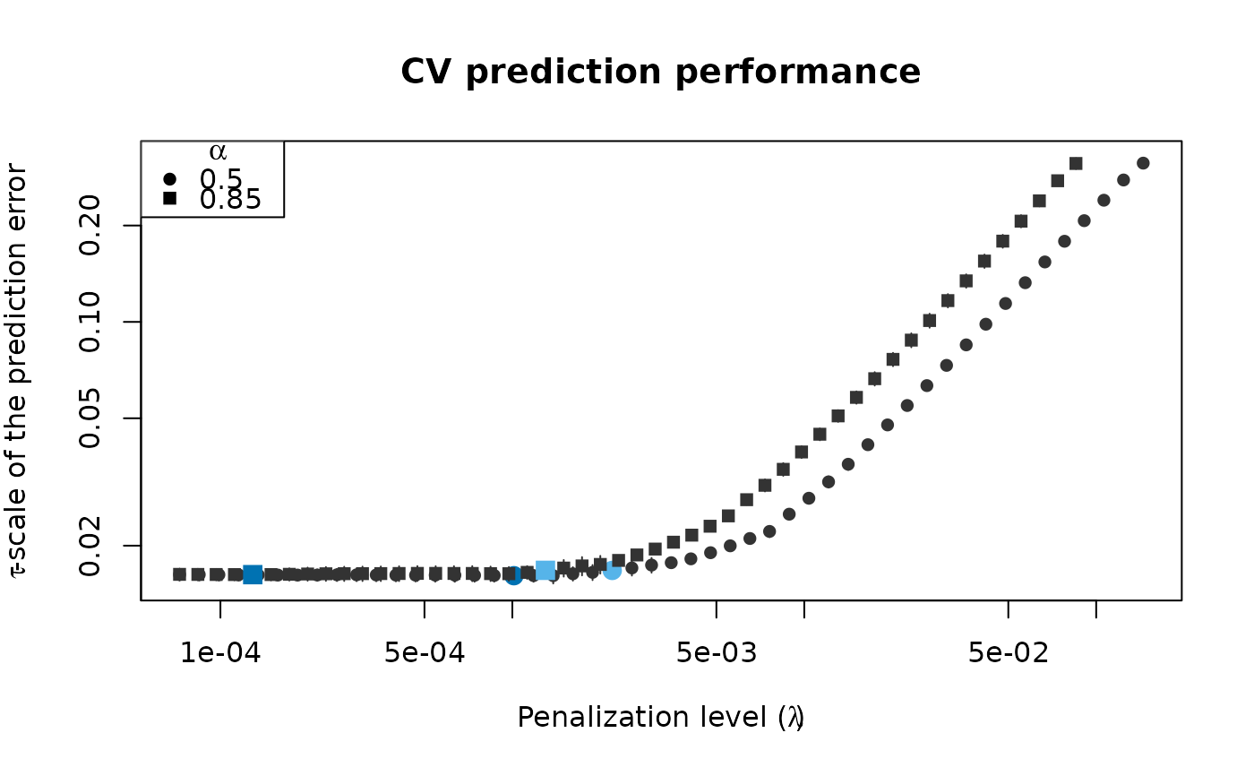
# What penalization level leads to good prediction performance?
set.seed(123)
cv_results <- regmest_cv(x, freeny$y, alpha = c(0.5, 0.85), scale = 2,
                         cv_repl = 2, cv_k = 4)
plot(cv_results, se_mult = 1)


# Print a summary of the fit and the cross-validation results.
summary(cv_results)
#> Regularized M fit with prediction performance estimated by replications of 
#> 4-fold cross-validation.
#> 
#> 4 out of 4 predictors have non-zero coefficients:
#> 
#>               Estimate
#> (Intercept) -9.1008312
#> X1           0.1900746
#> X2          -0.6944793
#> X3           0.7193090
#> X4           1.1802400
#> ---
#> 
#> Hyper-parameters: lambda=0.001012326, alpha=0.5

# Extract the coefficients at the penalization level with
# smallest prediction error ...
coef(cv_results)
#>           (Intercept) lag.quarterly.revenue           price.index 
#>            -9.1008312             0.1900746            -0.6944793 
#>          income.level      market.potential 
#>             0.7193090             1.1802400 
# ... or at the penalization level with prediction error
# statistically indistinguishable from the minimum.
coef(cv_results, lambda = '1-se')
#>           (Intercept) lag.quarterly.revenue           price.index 
#>            -8.7197254             0.2111671            -0.6634113 
#>          income.level      market.potential 
#>             0.6986596             1.1349456