Compute elastic net M-estimates along a grid of penalization levels with optional penalty loadings for adaptive elastic net.
Usage
regmest(
  x,
  y,
  alpha,
  nlambda = 50,
  lambda,
  lambda_min_ratio,
  scale,
  starting_points,
  penalty_loadings,
  intercept = TRUE,
  eff = 0.9,
  rho = "mopt",
  cc,
  eps = 1e-06,
  explore_solutions = 10,
  explore_tol = 0.1,
  max_solutions = 1,
  comparison_tol = sqrt(eps),
  sparse = FALSE,
  ncores = 1,
  standardize = TRUE,
  algorithm_opts = mm_algorithm_options(),
  add_zero_based = TRUE,
  mscale_bdp = 0.25,
  mscale_opts = mscale_algorithm_options()
)
Arguments
- x
nbypmatrix of numeric predictors.- y
vector of response values of length
n. For binary classification,yshould be a factor with 2 levels.- alpha
elastic net penalty mixing parameter with \(0 \le \alpha \le 1\).
alpha = 1is the LASSO penalty, andalpha = 0the Ridge penalty.- nlambda
number of penalization levels.
- lambda
optional user-supplied sequence of penalization levels. If given and not
NULL,nlambdaandlambda_min_ratioare ignored.- lambda_min_ratio
Smallest value of the penalization level as a fraction of the largest level (i.e., the smallest value for which all coefficients are zero). The default depends on the sample size relative to the number of variables and
alpha. If more observations than variables are available, the default is1e-3 * alpha, otherwise1e-2 * alpha.- scale
fixed scale of the residuals.
- starting_points
a list of staring points, created by
starting_point(). The starting points are shared among all penalization levels.- penalty_loadings
a vector of positive penalty loadings (a.k.a. weights) for different penalization of each coefficient. Only allowed for
alpha> 0.- intercept
include an intercept in the model.
- eff
the desired asymptotic efficiency of the M-estimator under the Normal model.
- rho
which \(\rho\) function to use (see
rho_function()for the list of supported options).- cc
manually specified cutoff constant for the chosen \(\rho\) function. If specified, overrides the
effargument.- eps
numerical tolerance.
- explore_solutions
number of solutions to compute up to the desired precision
eps.- explore_tol
numerical tolerance for exploring possible solutions. Should be (much) looser than
epsto be useful.- max_solutions
only retain up to
max_solutionsunique solutions per penalization level.- comparison_tol
numeric tolerance to determine if two solutions are equal. The comparison is first done on the absolute difference in the value of the objective function at the solution. If this is less than
comparison_tol, two solutions are deemed equal if the squared difference of the intercepts is less thancomparison_toland the squared \(L_2\) norm of the difference vector is less thancomparison_tol.- sparse
use sparse coefficient vectors.
- ncores
number of CPU cores to use in parallel. By default, only one CPU core is used. Not supported on all platforms, in which case a warning is given.
- standardize
logical flag to standardize the
xvariables prior to fitting the M-estimates. Coefficients are always returned on the original scale. This can fail for variables with a large proportion of a single value (e.g., zero-inflated data). In this case, either compute withstandardize = FALSEor standardize the data manually.- algorithm_opts
options for the MM algorithm to compute estimates. See
mm_algorithm_options()for details.- add_zero_based
also consider the 0-based regularization path in addition to the given starting points.
- mscale_bdp, mscale_opts
options for the M-scale estimate used to standardize the predictors (if
standardize = TRUE).
Value
a list-like object with the following items
alphathe sequence of
alphaparameters.lambdaa list of sequences of penalization levels, one per
alphaparameter.scalethe used scale of the residuals.
estimatesa list of estimates. Each estimate contains the following information:
interceptintercept estimate.
betabeta (slope) estimate.
lambdapenalization level at which the estimate is computed.
alphaalpha hyper-parameter at which the estimate is computed.
objf_valuevalue of the objective function at the solution.
statuscodeif
> 0the algorithm experienced issues when computing the estimate.statusoptional status message from the algorithm.
callthe original call.
See also
regmest_cv() for selecting hyper-parameters via cross-validation.
coef.pense_fit() for extracting coefficient estimates.
plot.pense_fit() for plotting the regularization path.
Other functions to compute robust estimates:
pense()
Examples
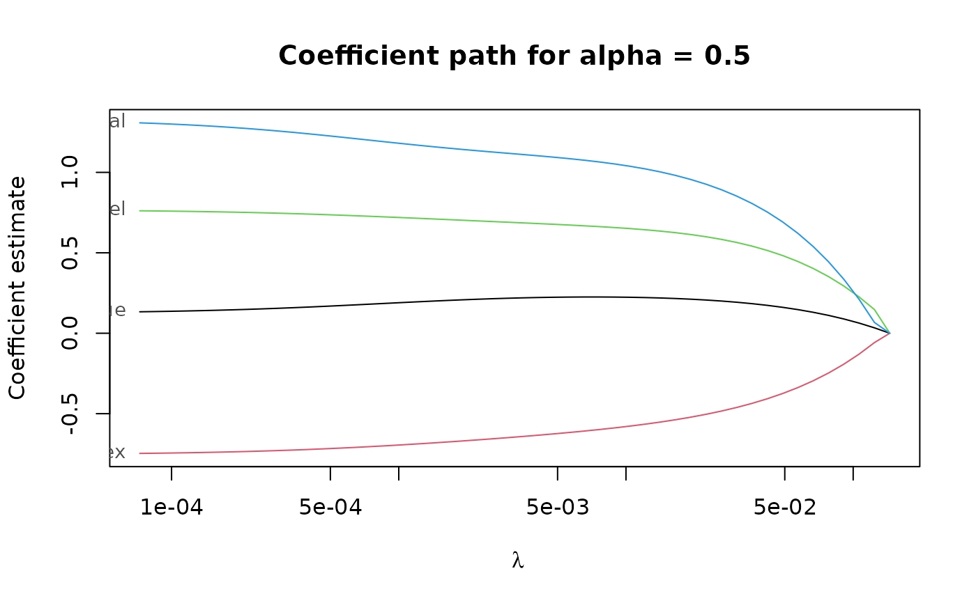
# Compute the PENSE regularization path for Freeny's revenue data
# (see ?freeny)
data(freeny)
x <- as.matrix(freeny[ , 2:5])
regpath <- regmest(x, freeny$y, alpha = c(0.5, 0.85), scale = 2)
plot(regpath)
 # Extract the coefficients at a certain penalization level
coef(regpath, alpha = 0.85, lambda = regpath$lambda[[2]][[40]])
#> (Intercept) lag.quarterly.revenue price.index
#> -9.9619795 0.1375927 -0.7438982
#> income.level market.potential
#> 0.7590060 1.2820779
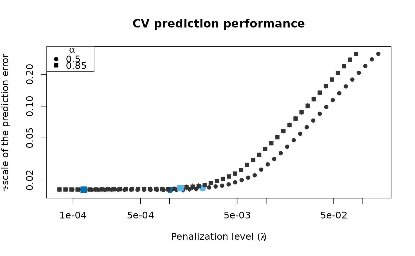
# What penalization level leads to good prediction performance?
set.seed(123)
cv_results <- regmest_cv(x, freeny$y, alpha = c(0.5, 0.85), scale = 2,
cv_repl = 2, cv_k = 4)
plot(cv_results, se_mult = 1)
# Extract the coefficients at a certain penalization level
coef(regpath, alpha = 0.85, lambda = regpath$lambda[[2]][[40]])
#> (Intercept) lag.quarterly.revenue price.index
#> -9.9619795 0.1375927 -0.7438982
#> income.level market.potential
#> 0.7590060 1.2820779
# What penalization level leads to good prediction performance?
set.seed(123)
cv_results <- regmest_cv(x, freeny$y, alpha = c(0.5, 0.85), scale = 2,
cv_repl = 2, cv_k = 4)
plot(cv_results, se_mult = 1)
 # Print a summary of the fit and the cross-validation results.
summary(cv_results)
#> Regularized M fit with prediction performance estimated by replications of
#> 4-fold cross-validation.
#>
#> 4 out of 4 predictors have non-zero coefficients:
#>
#> Estimate
#> (Intercept) -9.1008312
#> X1 0.1900746
#> X2 -0.6944793
#> X3 0.7193090
#> X4 1.1802400
#> ---
#>
#> Hyper-parameters: lambda=0.001012326, alpha=0.5
# Extract the coefficients at the penalization level with
# smallest prediction error ...
coef(cv_results)
#> (Intercept) lag.quarterly.revenue price.index
#> -9.1008312 0.1900746 -0.6944793
#> income.level market.potential
#> 0.7193090 1.1802400
# ... or at the penalization level with prediction error
# statistically indistinguishable from the minimum.
coef(cv_results, lambda = '1-se')
#> (Intercept) lag.quarterly.revenue price.index
#> -8.7197254 0.2111671 -0.6634113
#> income.level market.potential
#> 0.6986596 1.1349456
# Print a summary of the fit and the cross-validation results.
summary(cv_results)
#> Regularized M fit with prediction performance estimated by replications of
#> 4-fold cross-validation.
#>
#> 4 out of 4 predictors have non-zero coefficients:
#>
#> Estimate
#> (Intercept) -9.1008312
#> X1 0.1900746
#> X2 -0.6944793
#> X3 0.7193090
#> X4 1.1802400
#> ---
#>
#> Hyper-parameters: lambda=0.001012326, alpha=0.5
# Extract the coefficients at the penalization level with
# smallest prediction error ...
coef(cv_results)
#> (Intercept) lag.quarterly.revenue price.index
#> -9.1008312 0.1900746 -0.6944793
#> income.level market.potential
#> 0.7193090 1.1802400
# ... or at the penalization level with prediction error
# statistically indistinguishable from the minimum.
coef(cv_results, lambda = '1-se')
#> (Intercept) lag.quarterly.revenue price.index
#> -8.7197254 0.2111671 -0.6634113
#> income.level market.potential
#> 0.6986596 1.1349456